Analyzing Expensive Real-Time Task Models Inexpensively?

Originally, I planned to write something on this topic that is readable for a broader range of readers. Unfortunately, I realized this is beyond my capability as soon as I started writing. If you feel your time wasted by reading this post, please write me an email (nan.guan”at”polyu.edu.hk) to ask for a refund of your time. I will try my best to satisfy you, when technology allows. 😉

Two Parallel Paths to the Same Direction

Many real-time systems are safe-critical, so their timing correctness must be ensured under any circumstance at runtime. To guarantee this, we should describe the system behavior by some rigorous models, based on which properties of interests can be proved. Research on formal modeling and analysis of real-time systems has been done in, at least, two research areas: real-time scheduling and model-checking.

In real-time scheduling, people use simple abstractions, e.g., the Liu and Layland periodic task model, to describe a computing system, and develop efficient techniques to verify commonly concerned properties such as whether the deadlines are always honored. Of course, there is no clear standard of being “efficient”. Usually people in this field consider polynomial time (or even pseudo-polynomial time) analysis to be efficient, at least for off-line usage.

In model-checking, people use highly expressive formulas (e.g., various types of automata) to model a system. Some of these formulas are as expressive as Turing Machine, so one can almost describe anything that could happen in a computer with them, but on the other hand the general analysis problems are undecidable at all. By limiting their expressiveness we can bring them back to the decidable side, but their analysis problems are still in high positions in the complexity hierarchy. Exponential time complexity is standard in this world.

These two areas have been developing almost independently in the past several decades. There are some researchers having expertise in both areas and from time to time there are interesting papers combining insights of the two areas in some way. However, the overlapping of the two areas is still quite limited, compared with the large amount of research work conducted in each of them.

It is quite natural to ask, what is the fundamental difference between the theory and techniques in these two areas and, is it possible to establish a framework to unify them? Here I am discussing these problems purely for the sake of curiosity. If we want to discuss, for example, “why would we want to unify them in the first place”, or “would that be useful to better solve realistic problems”, that is another story.

The Model-Checking Myth

The model-checking techniques are ultimately delivered as tools usually called model-checkers, which provides the interface for the user to describe a system with the underlying model and properties of the model that they want to check, and an engine to automatically perform some kind of “searching” to check whether the properties hold. As soon as we have modelled the system and the concerned properties with a model-checker, the only thing we need to do is to click the “start” button of the model-checker and wait for it to give us the answer. Due to the high expressiveness of the underlying models, model-checkers appear to be extremely powerful tools, which can almost answer all their questions. The only problem is the long time it takes to produce the answer (and also the large amount of memory it consumes).

Model-checking is a large research area in which people work with many different models and different types of techniques. I try to summarize some of their common features based on my very limited knowledge. The models are usually state transition systems, which can be represented by some types of graphs. A vertex of the graph usually represents a state or a collection of states which share some similarities and an edge represents the transition from one state (set) to another, usually annotated with the conditions for the transition to happen and the consequence after taking this transition.

Given an input (e.g., a sequence of events that make certain conditions on the edges satisfied), we can “run” the model by transiting among the edges. The run is non-deterministic in the sense that given an input one may run the model in different ways (e.g., if an input event can trigger transitions along two outing edges of a vertex, then one can take any one of them arbitrarily). With these models, the goal is to check, given certain inputs, whether certain things (e.g., a state being visited) may or must happen, or may/must happen in some certain pattern, etc. To perform such checking, in principle we need to check all the possible runs of the model. Explicitly enumerating all the possible runs are computationally intractable (there could also be infinitely many possible runs and each run could be an infinite sequence). The magic of model-checking techniques is to perform such checking more “efficiently” (compared with the effort of explicit enumeration) even in the presence of infinity. People developed compact state representations, e.g., grouping (infinitely) many states in an equivalent class, and techniques to efficiently search over the possible runs with these compact state representations.

The Real-Time Scheduling Weapons

In real-time scheduling theory, a system is usually modeled by a collection of parameters and a well-defined scheduling policy. Take the well-known Liu and Layland’s periodic task model as the example. A system is a collection of independent tasks, each characterized by a period T and a worst-case execution time (WCET) C. A task repeatedly release jobs at a minimum separation of T time units and each job executes for at most C time units. If the task system is scheduled by RM (rate-monotonic) scheduling policy, in which a task with a shorter period always has higher priority than (and thus can preempt) those with longer periods, it is proved that all jobs of all tasks can meet their deadlines if the summation of C/T of all tasks is no larger than ln2 (we call this constant ln2 the utilization bound). The utilization bound is 1, instead of ln2, if the task set is scheduled by another scheduling policy EDF (earliest-deadline-first). Over years, Liu and Layland’s periodic task model has been extended to express more complex timing behaviors of the tasks.

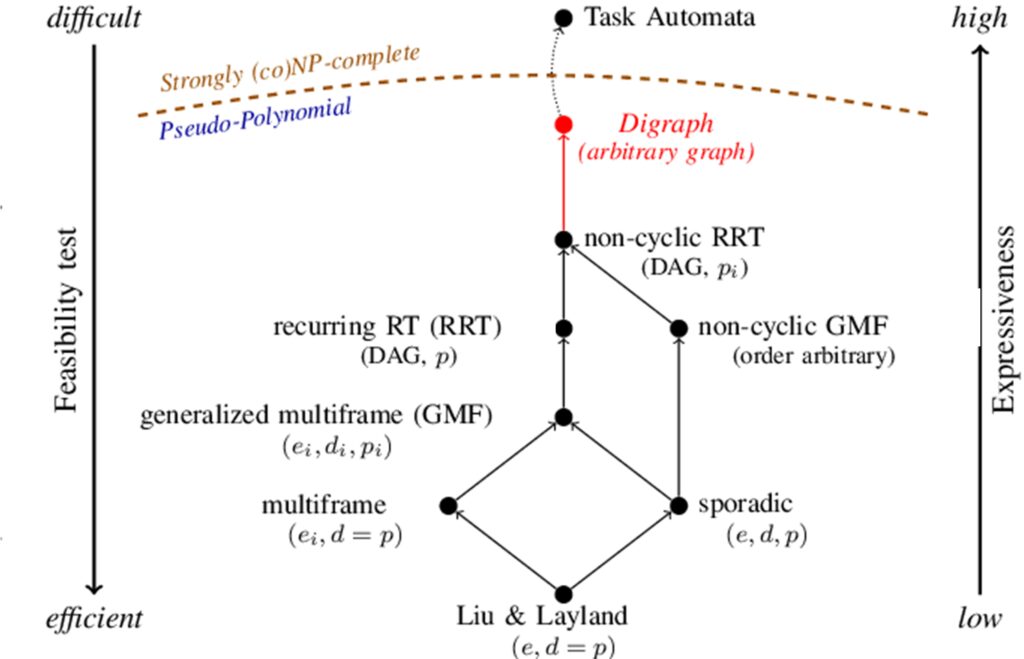The left figure (due to Martin Stigge) shows the extension of the models in a particular dimension concerning the workload release pattern. Notably, many of these models use graph structures, which already looks somehow similar to those in model-checking. However, the analysis techniques developed for them in real-time scheduling theory is very different from, and significantly more efficient than in model-checking. For example, the analysis of the Digraph task model under EDF scheduling has a pseudo-polynomial time complexity, and can scale to thousands of and even more tasks with graph structures of tens and even hundreds of vertices. However, if we use the model-checking techniques to model and analyze them (e.g., using a state-of-the-art model-checker UPPAAL), the scalability ceiling could be several tasks with several vertices in each task graph.

What is the key to make the efficiency of real-time scheduling analysis so much higher than model-checking? The high-level answer is, of course, the restrictive expressiveness of the task models in real-time scheduling (even if some of them are already not so restrictive). We could have a closer look and think of whether there are any insights that we could borrow from the analysis techniques in real-time scheduling to significantly improve the efficiency of model-checking, at least for those models/properties that are more similar to those in real-time scheduling.

I try to understand what gives the high efficiency of real-time scheduling analysis. In my opinion, there are at least three key contributors.

Busy Periods. Real-time tasks are typically recurrently activated, which leads to very large (even infinite) state space. Instead of looking into the whole state space of the system, many real-time scheduling analysis techniques focus on the so-called busy period, which refers to the maximal continuous time intervals during which the task under analysis has backlogged workload. If the task under analysis misses its deadline, it occurs within a busy period. This greatly reduces the state space to be checked. The concept of busy periods and the information implied in different real-time scheduling analysis problems are different. In some problems, the busy period can be very precisely characterized. In some other problems, the busy period can only be approximately characterized.  Nevertheless, even with those vague busy period concepts, the state-space of the system can still be greatly reduced compared with looking into the whole time horizon.

Workload Abstractions. Even if the analysis is limited into busy periods, the state space may still be very large. In real-time scheduling analysis, instead of explicitly encoding and checking the state space, numerical abstractions are used to compactly represent and system behavior. For example, many real-time scheduling analysis techniques use demand bound functions (DBF) to characterize the largest amount of workload of a task that must be finished in a time interval of certain length. To check schedulability, it is sufficient to calculate the total amount of work to finish before particular time points, in order to decide whether dead misses would occur. This greatly abstracts away unnecessarily detailed behavior information of the system, e.g., which task is executing at a particular time point, and the verification is reduced to efficient manipulations of the numerical abstractions of individual tasks (e.g., summing up the DBF of each individual task to get the total DBF of the entire system).

Over-approximation. Although in general real-time task models are much less expressive and thus the analysis problems are much easier than in model-checking, many real-time scheduling analysis problems can still be hard (e.g., strongly NP-hard). In these cases, people may resort to over-approximation, e.g., calculating safe upper bounds of the response time (instead of calculating the precise one) or deriving sufficient schedulability test conditions (instead of deriving the sufficient and necessary conditions). Approximate analysis is false positive: it may pessimistically claim a correct system to be incorrect, and requires the designer to provide more resources than necessary, but will never overlook systems that are indeed incorrect.

Analyzing Expensive Models Inexpensively

Can we develop some efficient analysis framework for complex task systems that are modeled with those expressive models? For example, let’s consider timed automata, a widely used model for describing timed systems. Essentially, timed automata are finite state machines extended with clocks variables representing the elapse of time.

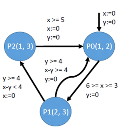The left figure shows a simple timed automaton (extended with semantics of workload release), where the system runs by switching among the three vertices. Each vertex (P0, P1 or P2) is annotated with job information described by two parameters, the WCET and the relative deadline. When the system enters a vertex, a job is released correspondingly. Switching among different vertices is constrained by the conditions regarding the two clock variables x and y. The system initially starts by entering vertex P0 and both x and y are initialized to be 0. When the system states in P0, time elapses, i.e., both clocks continuously increase at the same rate. Then the system can take the transition from P0 to P1 when x is in the range [3, 6], and when taking this transition y is reset to be 0. In general, a timed automaton may use many clock variables to describe extremely complex workload release behaviors.

Now consider a task system consisting of several independent tasks, each modeled by a timed automata, and we ask whether the system is schedulable under, e.g.,  EDF scheduling algorithm. To answer this, we can use model-checkers, e.g., UPPAAL or TimesTool to build a timed automata network, which consists of timed automata encoding the tasks plus an extra timed automaton encoding the resource sharing among them under the given scheduling policy. The schedulability is checked by verifying whether the system may go into a state where some released job cannot be finished before its deadline.

Hopefully we may be able to analyze the schedulability of such a task model much more efficiently with the analysis technique framework of real-time scheduling theory. Suppose the tasks are scheduled by EDF. If we can compute the DBF of each individual task, then we can check the system schedulability in essentially the same way as the simple real-time task models: adding up the DBF of all tasks and check whether its exceeds the resource availability. In this case, DBF is a very good abstraction telling how much resource is required in certain time internals for each task to meet the deadline. By computing the DBF, we directly focus on the most important aspect on the right level of abstraction, without looking into the details, e.g., which task executes at a time point exactly.

Computing the DBF of an individual timed automata may still be quite expensive. Essentially we need to explore all the possible paths of the timed automata graph. However, it is still much better than the ordinary model-checking approach. This is because, with the DBF-based approach, we only need to deal with the complexity of each task separately — after obtaining the DBF of each individual task, checking schedulability of the whole system becomes easy (simply adding up the DBF of all tasks). In contrast, with the original model-checking approach, we first compute the production of all timed automata and the extra “scheduler” automata, which is a large timed automaton with exponential size with respect to the number of tasks, and then perform “searching” on this large timed automaton. Note that, although we assume the tasks are “independent” (in the sense that their release times, execution times, deadlines and so on do not rely on each other), they are actually not, because they have to interact with each other by sharing CPU time. Therefore, the ordinary model-checking approach has to compute the production of all timed automata to capture such interaction.

Of course, in general, it may not always be possible to perfectly decouple the analysis of the whole system into efficient analysis of individual tasks as in the above simple example. Nevertheless, the central idea of the busy-period-based analysis in real-time scheduling theory is exactly to do such composition, so hopefully many techniques developed in this area would be useful to analyze the expressive models in a more compositional manner. For example, if the tasks share not only the CPU, but also some other logical and physical shared resource (e.g., protected by locks), then it may be possible to reuse or extend the techniques of blocking-time computation in real-time scheduling theory, and add the blocking time to the DBF when analyzing the schedulability of each individual task. As long as we accept over-approximate analysis, the DBF-based framework can be enhanced by adding different extra factors to handle much more complex cases.

Author bio: Nan Guan is currently an associate professor at The Hong Kong Polytechnic University. His research interests include real-time scheduling, formal verification, system software and their applications in embedded systems, cyber-physical systems (CPS) and Internet-of-things (IoT). He has great potential to become a good blog writer.